I read with interest a recent post at Online Behavior on Visualizing Google Analytics Data With R and thought I would share my own Shiny application for visualising visits, bounce rate etc. from a website which I contributed to. The website is dedicated to sharing the feedback about Nottinghamshire Healthcare NHS Trust and the action which the Trust has taken from the feedback: the Your Feedback Matters site.
This application features in my book Web application development with R using Shiny which is a complete introduction to Shiny, a free package available for R. For those who are not familiar with Shiny, it greatly simplifies the production of interactive web interfaces for exploring data using R.
Here is a screenshot from my sample application, you can interact with the data here.

Shiny includes a range of functions which handle the styling of the page, the production of input widgets within the interface, and uses a Reactive programming paradigm to ensure that calls to graphs and other outputs are based on the inputs and data the user has requested most recently, automatically updating background calculations and outputs as the user selects different input values within the interface. Shiny applications can be written as pure R code but Shiny is very extensible, allowing those with the requisite knowledge to use HTML, CSS, JavaScript, and jQuery (demos here) to build and style the application exactly how they want it.
All of the code and data for the application lives on GitHub here, and if you wish to demo the application just install the Shiny package within R and run the following on your console:
library(shiny)

runGitHub("GoogleAnalytics", "ChrisBeeley")
Shiny applications are made of two code files which are placed in the same directory, ui.R and server.R. The ui.R code file defines the interface, what the input widgets are and how they work, the types of output which will be displayed and their layout, etc. The server.R file does all the data processing and produces the graphs, tables, and other outputs that are then arranged by the code in the ui.R file. To give you a flavour of how it fits together I will summarise snippets from each, for more details look at the Shiny documentation at the link to Shiny above, browse the code on GitHub or read my book.
The ui.R file begins thus:
###################################

##### Google Analytics - ui.R #####

###################################
library(shiny)
shinyUI(pageWithSidebar(
headerPanel("Google Analytics"),
sidebarPanel(
dateRangeInput(inputId = "dateRange",
label = "Date range",
start = "2013-04-01",
max = Sys.Date()
),
shinyUI(pageWithSidebar())gives the most common Shiny layout, with widgets on the left and outputs on the right, although there are other options and you can produce the whole thing in HTML if you wish.headerPanel()gives a nice big title at the top.sidebarPanel()command describes all the widgets. The first, as you can see, is a date widget which allows you to use a friendly calendar like interface to select a minimum and maximum date.
Other examples within this example include:
sliderInput(inputId = "maximumTime",

  label = "Hours of interest- maximum",

  min = 0,

  max = 23,

  value = 23,

  step = 1)
Which gives a slider for selecting numerical values with (in this case, hours from a 24 hour clock, and:
checkboxInput(inputId = "smoother",

  label = "Add smoother?",

  value = FALSE)
Which gives a checkbox which allows users to specify whether they want a smoothing line on their graph or not. In both cases you can see they are given an inputID value, this allows the server.R file to pick up values from these widgets using input$…, e.g. input$dateRange or input$maximumTime.
The ui.r file ends by defining the output region like this:
mainPanel(

  tabsetPanel(

    tabPanel("Summary", textOutput("textDisplay")),

    tabPanel("Monthly figures", plotOutput("monthGraph")),

    tabPanel("Hourly figures", plotOutput("hourGraph"))

  )
The tabsetPanel() function allows you to have multiple output pages selectable by tabs, and as you can see the tabPanel() function gives them a name to be displayed to the user and a name to associate them with the outputs in the server.R file.
The server.R file processes the data according to user inputs and prepares the output. The data is processed in a reactive function according to the reactive programming paradigm alluded to earlier – that is to say when the inputs change, the data changes. The function looks like this:
passData <- reactive({

analytics <- analytics[analytics$Date %in%
  seq.Date(input$dateRange[1],
  input$dateRange[2], by = "days"), ]

analytics <- analytics[analytics$Hour %in%
  as.numeric(input$minimumTime):
  as.numeric(input$maximumTime), ]

analytics
})
As you can see the data is prepared according to the values of input$dateRange and input$maximumTime that we saw earlier. The final line simply reads "analytics" to indicate to Shiny that we wish the reactive function to return the object "analytics".
This dataframe can now be used anywhere it is needed in with the usual R indexing of dataframes applying, except two brackets are placed after analytics, e.g. passData()$variableName or passData()[,2:10]. The monthly graph can now be returned like this:
output$monthGraph <- renderPlot({

graphData <- ddply(passData(), .(Domain, Date), numcolwise(sum))

if(input$outputType == "visitors"){

  theGraph <- ggplot(graphData,
    aes(x = Date, y = visitors, group = Domain, colour = Domain)) +
    geom_line() + ylab("Unique visitors")

}

[... other types of graph- bounce rate, time on site]

print(graphData)
})
As you can see passData() is munged using the ddply command from the plyr package and then plotted very simply using ggplot2. You will notice also that this command is assigned to output$monthGraph, this is the ID we encountered before when setting up the outputs in the ui.R panel:
tabPanel("Monthly figures", plotOutput("monthGraph"))
Closing Thoughts
This has been a very brief tour of and introduction to using Shiny with Google Analytics data, do browse the GitHub and download the code and data to get a better feel for it, there is another version with advanced features (rather silly advanced features, I should say, they were written for educational purposes for the book and are not supposed to be directly useful as such), and do feel free to come visit my blog or find me on Twitter.