A/B testing is the field of digital marketing with the highest potential to apply scientific principles, as each A/B experiment is a randomized controlled trial, very similar to ones done in physics, medicine, biology, genetics, etc. However, common advice and part of the practice in A/B testing are lagging by about half a century when compared to modern statistical approaches to experimentation. There are major issues with the common statistical approaches discussed in most A/B testing literature and applied daily by many practitioners. The three major ones are:
- Misuse of statistical significance tests
- Lack of consideration for statistical power
- Significant inefficiency of statistical methods
In this article I discuss each of the three issues discussed above in some detail, and propose a solution inspired by clinical randomized controlled trials, which I call the AGILE statistical approach to A/B testing.
1. Misuse of Statistical Significance Tests
In most A/B testing content, when statistical tests are mentioned they inevitably discuss statistical significance in some fashion. However, in many of them a major constraint of classical statistical significance tests, e.g. the Student’s T-test, is simply not mentioned. That constraint is the fact that you must fix the number of users you will need to observe in advance.
Before going deeper into the issue, let’s briefly discuss what a statistical significance test actually is. In most A/B tests it amounts to an estimation of the probability of observing a result equal to or more extreme than the one we observed, due to the natural variance in the data that would happen even if there is no true positive lift.
Below is an illustration of the natural variance, where 10,000 random samples are generated from a Bernoulli distribution with a true conversion rate at 0.50%.
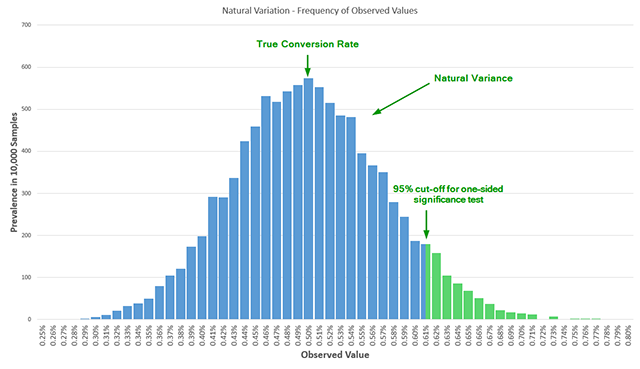
In an A/B test we randomly split users in two or more arms of the experiment, thus eliminating confounding variables, which allows us to establish a causal relationship between observed effect and the changes we introduced in the tested variants. If after observing a number of users we register a conversion rate of 0.62% for the tested variant versus a 0.50% for the control, that means that we either observed a rare (5% probability) event, or there is in fact some positive difference (lift) between the variant and control. In general, the less likely we are to observe a particular result, the more likely it is that what we are observing is due to a genuine effect, but applying this logic requires knowledge that is external to the statistical design so I won’t go into details about that. The above statistical model comes with some assumptions, one of which is that you observe the data and act on it at a single point in time. For statistical significance to work as expected we must adhere to a strict application of the method where you declare you will test, say, 20,000 users per arm, or 40,000 in total, and then do a single evaluation of statistical significance. If you do it this way, there are no issues. Approaches like “wait till you have 100 conversions per arm” or “wait till you observe XX% confidence” are not statistically rigorous and will probably get you in trouble. However, in practice, tests can take several weeks to complete, and multiple people look at the results weekly, if not daily. Naturally, when results look overly positive or overly negative they want to take quick action. If the tested variant is doing poorly, there is pressure to stop the test early to prevent losses and to redirect resources to more prospective variants. If the tested variant is doing great early on, there is pressure to suspend the test, call the winner and implement the change so the perceived lift can be converted to revenue quicker. I believe there is no A/B testing practitioner who will deny these realities. These pressures lead to what is called data peeking or data-driven optional stopping. The classical significance test offers no error guarantees if it is misused in such a manner, resulting in illusory findings – both in terms of direction of result (false positives) and in the magnitude of the achieved lift. The reason is that peeking results in an additional dimension in the test sample space. Instead of estimating the probability of a single false detection of a winner with a single point in time, the test would actually need to estimate the probability of a single false detection at multiple points in time. If the conversion rates were constant that would not be an issue. But since they vary without any interventions, the cumulative data varies as well, so adjustments to the classical test are required in order to calculate the error probability when multiple analyses are performed. Without those adjustments, the nominal or reported error rate will be inflated significantly compared to the actual error rate. To illustrate: peeking only 2 times results in more than twice the actual error vs the reported error. Peeking 5 times results in 3.2 times larger actual error vs the nominal one. Peeking 10 times results in 5 times larger actual error probability versus nominal error probability. This is known to statistical practitioners as early as 1969 and has been verified time and again. If one fails to fix the sample size in advance or if one is performing multiple statistical significance tests as the data accrues, then we have a case of GIGO, or Garbage In, Garbage Out.
2. Lack of Consideration for Statistical Power
In a review of 7 influential books on A/B testing published between 2008 and 2014 we found only 1 book mentioning statistical power in a proper context, but even there the coverage was superficial. The remaining 6 books didn’t even mention the notion. From my observations, the situation is similar when it comes to most articles and blog posts on the topic.
But what is statistical power and why is it important for A/B experiments? Statistical power is defined as the probability to detect a true lift equal to or larger than a given minimum, with a specified statistical significance threshold. Hence the more powerful a test, the larger the probability that it will detect a true lift. I often use “test sensitivity” and “chance to detect effect” as synonyms, as I believe these terms are more accessible for non-statisticians while reflecting the true meaning of statistical power.
Running a test with inadequately low power means you won’t be giving your variant a real chance at proving itself, if it is in fact better. Thus, running an under-powered test means that you spend days, weeks and sometimes months planning and implementing a test, but then failing to have an adequate appraisal of its true potential, in effect wasting all the invested resources. What’s worse, a false negative can be erroneously interpreted as a true negative, meaning you will think that a certain intervention doesn’t work while in fact it does, effectively barring further tests in a direction that would have yielded gains in conversion rate.
Power and Sample Size
Power and sample size are intimately tied: the larger the sample size, the more powerful (or sensitive) the test is, in general. Let’s say you want to run a proper statistical significance test, acting on the results only once the test is completed. To determine the sample size, you need to specify four things: historical baseline conversion rate (say 1%), statistical significance threshold, say 95%, power, say 90%, and the minimum effect size of interest. Last time I checked, many of the free statistical calculators out there won’t even allow you to set the power and in fact silently operate at 50% power, or a coin toss, which is abysmally low for most applications. If you use a proper sample size calculator for the first time you will quickly discover that the required sample sizes are more prohibitive than you previously thought and hence you need to compromise either with the level of certainty, or with the minimum effect size of interest, or with the power of the test. Here are two you could start with, but you will find many more on R packages, GPower, etc:
Making decisions about the 3 parameters you control – certainty, power and minimum effect size of interest is not always easy. What makes it even harder is that you remain bound to that one look at the end of the test, so the choice of parameters is crucial to the inferences you will be able to make at the end. What if you chose too high a minimum effect, resulting in a quick test that was, however, unlikely to pick up on small improvements? Or too low an effect size, resulting in a test that dragged for a long time, when the actual effect was much larger and could have been detected much quicker? The correct choice of those parameters becomes crucial to the efficiency of the test.
3. Inefficiency of Classical Statistical Tests in A/B Testing Scenarios
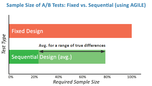
Classical tests are good in some areas of science like physics and agriculture, but are replaced with a newer generation of testing methods in areas like medical science and bio-statistics. The reason is two-fold. On one hand, since the hypotheses in those areas are generally less well defined, the parameters are not so easily set and misconfigurations can easily lead to over or under-powered experiments. On the other hand – ethical and financial incentives push for interim monitoring of data and for early stopping of trials when results are significantly better or significantly worse than expected. Sounds a lot like what we deal with in A/B testing, right? Imagine planning a test for 95% confidence threshold, 90% power to detect a 10% relative lift from a baseline of 2%. That would require 88,000 users per test variant. If, however, the actual lift is 15%, you could have ran the test with only 40,000 users per variant, or with just 45% of the initially planned users. In this case if you were monitoring the results you’d want to stop early for efficacy. However, the classical statistical test is compromised if you do that. On the other hand, if the true lift is in fact -10%, that is whatever we did in the tested variant actually lowers conversion rate, a person looking at the results would want to stop the test way before reaching the 88,000 users it was planned for, in order to cut the losses and to maybe start working on the next test iteration. What if the test looked like it would convert at -20% initially, prompting the end of the test, but that was just a hiccup early on and the tested variant was actually going to deliver a 10% lift long-term?
The AGILE Statistical Method for A/B Testing
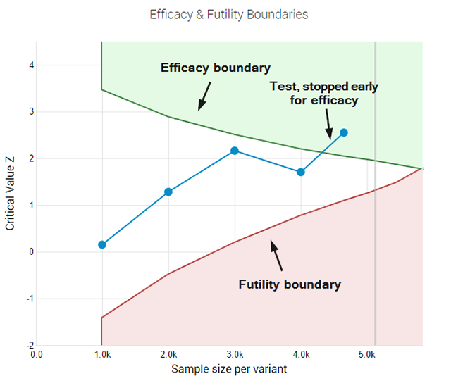
Questions and issues like these prompted me to seek better statistical practices and led me to the medical testing field where I identified a subset of approaches that seem very relevant for A/B testing. That combination of statistical practices is what I call the AGILE statistical approach to A/B testing. I’ve written an extensive white-paper on it called “Efficient A/B Testing in Conversion Rate Optimization: The AGILE Statistical Method”. In it I outline current issues in conversion rate optimization, describe the statistical foundations for the AGILE method and describe the design and execution of a test under AGILE as an easy step-by-step process. Finally, the whole framework is validated through simulations. The AGILE statistical method addresses misuses of statistical significance testing by providing a way to perform interim analysis of the data while maintaining false positive errors controlled. It happens through the application of so-called error-spending functions which results in a lot of flexibility to examine data and make decisions without having to wait for the pre-determined end of the test. Statistical power is fundamental to the design of an AGILE A/B test and so there is no way around it and it must be taken into proper consideration. AGILE also offers very significant efficiency gains, ranging from an average of 20% to 80%, depending on the magnitude of the true lift when compared to the minimum effect of interest for which the test is planned. This speed improvement is an effect of the ability to perform interim analysis. It comes at a cost since some tests might end up requiring more users than the maximum that would be required in a classical fixed-sample test. Simulations results as described in my white paper show that such cases are rare. The added significant flexibility in performing analyses on accruing data and the average efficiency gains are well worth it. Another significant improvement is the addition of a futility stopping rule, as it allows one to fail fast while having a statistical guarantee for false negatives. A futility stopping rule means you can abandon tests that have little chance of being winners without the need to wait for the end of the study. It also means that claims about the lack of efficacy of a given treatment can be made to a level of certainty, permitted by the test parameters. Ultimately, I believe that with this approach the statistical methods can finally be aligned with the A/B testing practice and reality. Adopting it should contribute to a significant decrease in illusory results for those who were misusing statistical tests for one reason or another. The rest of you will appreciate the significant efficiency gains and the flexibility you can now enjoy without sacrifices in terms of error control.

